


Tomorrow, October 17th, is #SpreadsheetDay. What will you be doing to celebrate? pic.twitter.com/5886ZXxF59
— Google Docs (@googledocs) October 16, 2015
In honor of spreadsheet day here are a few things to up your spreadsheet skills. I am including a spreadsheet template to try them out.
Template
1) Not For Numbers
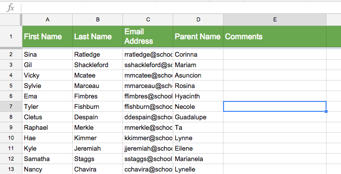
While spreadsheets are amazing for calculating numbers, you do not need to use any numbers to use spreadsheets. Spreadsheets are perfect for organizing information! Unless you are writing an essay, your default document type should be a spreadsheet.
Try It
On the first tab type in some comments for students in the list.
2) Comments
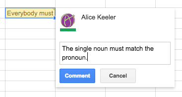
The only thing better than a spreadsheet is a collaborative spreadsheet. Google Sheets allows you to collaborate on a spreadsheet, which means you can also insert comments to facilitate collaboration.
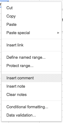
Right click on a cell or use the keyboard shortcut Control Alt M to insert a comment.
Try It
On the 2nd tab, insert comments to notify the collaborator that they have grammar errors.
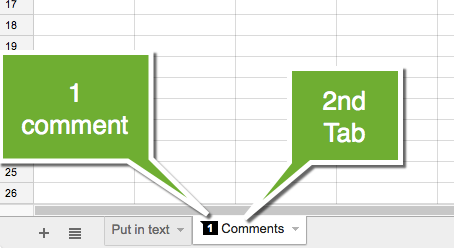
On the tab is a count of the number of comments on the sheet.
Note: When you make a copy of a spreadsheet, the comments do not copy. Use insert note instead of insert comment for ideas that need to be contained in copied documents.
3) Create a Hyperlink
A hyperlink is text that when you click on it, links to another website. If you type a website URL into a cell it will automatically create a hyperlink. However, a web URL tends to be long and does not fit nicely into a cell. Creating linked text can make for a more attractive spreadsheet that more clearly communicates the destination of the hyperlink.
Type text into a cell. Single click on the cell to select the cell. Use the chain link icon in the toolbar or use the keyboard shortcut Control K to create a hyperlink.
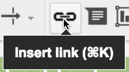
Google Sheets will attempt to predict the URL you wish to use. The hyperlink dialogue box has 2 boxes. The top box is the text that will appear in the cell. The bottom box is the link address. Paste the destination URL or choose from the drop down of predicted options.

Try It
On the 3rd tab named “Hyperlink” click on each text cell and hyperlink the text to the corresponding website. Google Sheets should predict the website without you having to look up the web addresses.
Note: While in edit mode of a spreadsheet, hyperlinks require 2 clicks. Clicking on the linked text will display the destination URL either above or below the text. Click on that hyperlink to launch the website. In published view, the hyperlinks work as a single click.

4) Duplicate Data
One advantage to using a spreadsheet is you can avoid having to update the same information in multiple places. Using cell referencing, when you make one change, other occurrences of that information can be updated.
For teachers, one example of this is a class roster. Oftentimes I need to have a list of student names on more than one sheet. I have a list of student names I type once. Any other instances of students names I will reference the original list.
To reference a cell, click on a blank cell and type an equals sign. Either click on the referenced cell or type the cell address. For example =A5 will put the value of A5 in the new cell.
Try It
On the 4th tab, named “Names again,” use cell referencing to insert the list of names from the first tab. In cell A2 type an equals sign. Go to the “Put in text” tab and click on cell A2. Press enter. If cell A2 is covered, click on a different cell and edit the cell address. 
In cell A2 of the “Names again” tab, the cell reference should be
=‘Put in text’!A2
Note: You do not have to individually reference each cell. Spreadsheets pick up patterns. Click on cell A2 and notice the fill down square in the bottom right-hand corner. Click and hold down on the square. Pull DOWN to continue the pattern down the sheet. Pull to the RIGHT to continue the pattern to the right.
5) Named Ranges
For those of you who are already spreadsheet ninjas this tip is for you. Jonathan Rochelle (@jrochelle) taught me this trick to name ranges. Naming ranges allows you to refer to a range of cells by a name in a spreadsheet rather than the range address.
For example instead of =vlookup(A2,$D$5:F:15,3)
Name the range D5:F15 as “Table.”
The new formula becomes =vlookup(A2,Table,3)
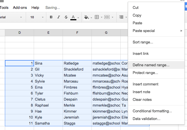
To name a range, highlight the range and right click. Choose “Define named range…” Choose a name for the range. When writing formulas type the named range in place of the range address. No quotation marks needed.
Try It
On the 5th tab, named “Named Range,” highlight the table of data. Right click and choose “Define named range…” Choose a name. Double click on cell B2 to edit the formula. Replace the range with the named range.


1 thought on “Spreadsheet Day – 5 Tips for Google Sheets”
I love these spreadsheet tips! Once again, my nerd status confirmed…